
Demo Game Slot Online RTP TinggiDemo Game Slot Online RTP Tinggi
Demo Game Slot Online RTP Tinggi – Game slot online merupakan permainan arcade terpopuler yang cocok untuk seluruh pemain. Cara

Demo Game Slot Online RTP Tinggi – Game slot online merupakan permainan arcade terpopuler yang cocok untuk seluruh pemain. Cara
Layanan Pencadangan Online Upload Tercepat 2023 – Tergantung pada apa Anda menggunakan pencadangan online, kecepatan dapat menjadi sangat penting atau
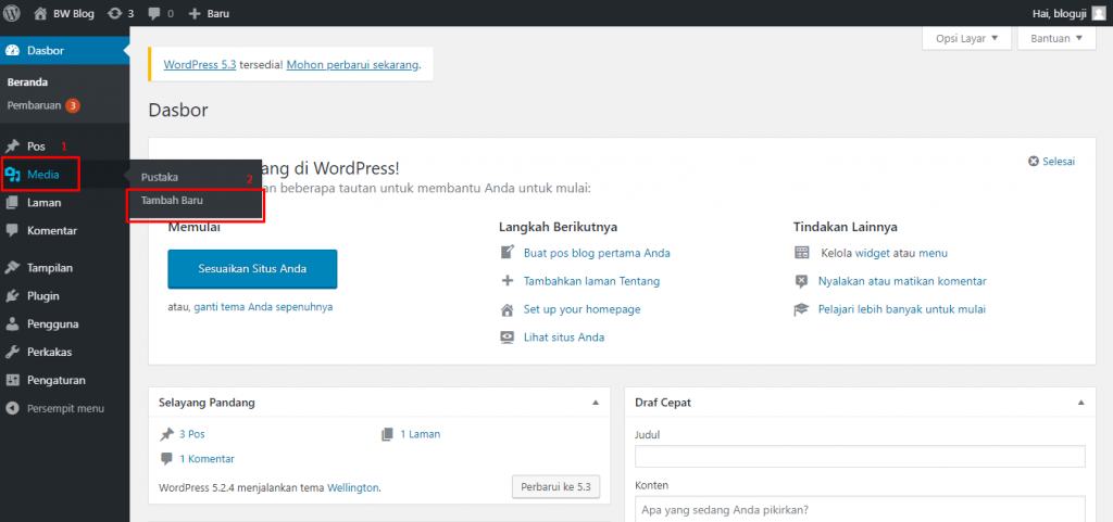
Cara Upload File ke Website – Sebelum file apa pun dapat dilihat di situs web melalui Internet, Anda perlu mengunggah
Simak Penjelasan Cara upload file ke internet – Saat browser Internet mengunjungi situs web Anda, hal pertama yang dilakukannya adalah mencari
5 Situs Berbagi File Gratis Terbaik Dan Program Perangkat Lunak 2023 – Situs berbagi file menyediakan layanan untuk mengakses media digital

Simak Penjelasan Tentang Kerentanan pengunggahan file – Di bagian ini, Anda akan mempelajari bagaimana fungsi pengunggahan file sederhana dapat digunakan sebagai

10 tips unggah file HTML yang berguna untuk pengembang web – Kemampuan untuk mengunggah file merupakan persyaratan utama untuk banyak aplikasi

5 Solusi Pengunggah File Terbaik di 2023 – Solusi Pengunggah File adalah aplikasi berbasis web yang memungkinkan Anda membuat dan berbagi
Cara Transfer File Melalui Wi-Fi Antara PC Dengan PC Lain Dan Smartphone – Transfer file Wi-Fi telah mendapatkan popularitas sebagai

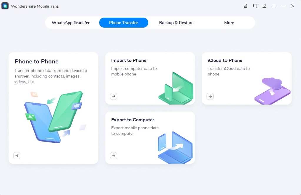
6 Cara Mentransfer File Dari PC Ke Ponsel Android Secara Nirkabel – Beberapa waktu lalu, saya ingin mentransfer beberapa file

Bahaya Keamanan Teratas Saat Mengunggah File Dan Cara Mencegahnya – Unggahan file merupakan bagian integral dari sistem dan layanan apa
Apa Itu File Transfer Protocol (FTP) Dan Apa Kegunaannya? – Istilah protokol transfer file (FTP) mengacu pada proses yang melibatkan
Ulasan Aplikasi Share File Xender: Aplikasi Upload File Tercepat – Xender adalah aplikasi yang menggunakan teknologi wifi untuk mentransfer file
Upload File Di Codeigniter Dengan Source Code – Upload A File In Codeigniter adalah sistem berbasis web yang berfungsi penuh.
9 Aplikasi Unggah File Terbaik untuk iOS yang Anda Butuhkan Sekarang – Dalam dunia yang terhubung yang kita tinggali, kita
Aplikasi File Unggah Shopify Terbaik di 2022 – Anda adalah pengusaha yang sibuk menjalankan bisnis e-niaga Anda, dan meneliti aplikasi

Mengatasi Tidak Dapat Mengunggah File ke Google Drive? – Google Drive adalah salah satu alat terpenting di gudang pekerja komputer

Unggah File AJAX – Tutorial Cepat & Tip Hemat Waktu – Unggah file melalui teknik AJAX dapat menjadi hal yang

Skrip Pengunggahan dan Berbagi File PHP Terbaik – Sebagian besar aplikasi web yang tersedia saat ini mencakup kemampuan pengguna untuk
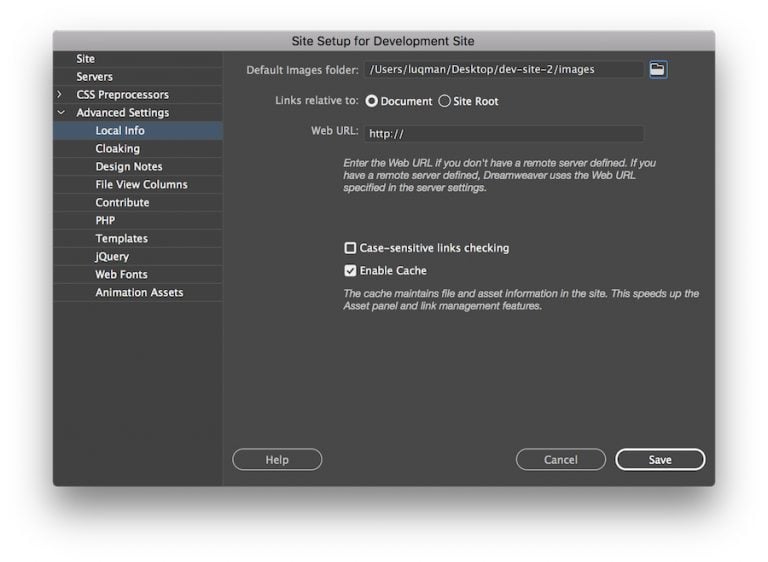
Cara Mengunggah File ke Situs Web Anda Menggunakan WinSCP – Untuk mengunggah file dari komputer Anda ke situs web Anda,
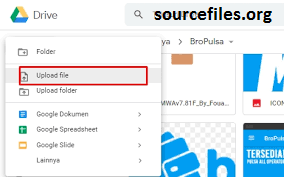
Cara Mengunggah ke Google Drive pada tahun 2022: Memindahkan File Anda ke Cloud – Mendapatkan akses ke 15GB ruang penyimpanan

Unggah File Vb Ke Server Web – File ini dimulai dengan baris yang mengidentifikasinya sebagai daftar file. Bagaimana menambahkan dialog
8 Situs Berbagi File Aman untuk Mengunggah, Menyimpan & Mentransfer File! – Apakah Anda mencari situs berbagi file gratis ?
Aplikasi Unggah File Terbaik untuk iOS yang Anda Butuhkan Sekarang – Dalam dunia yang terhubung yang kita tinggali, kita sering

Unggah dari URL, Dropbox, Google Drive, dan Sumber Lainnya – Uploadcare adalah File API lengkap yang menyediakan penanganan file tanpa

Kirim File Besar Dengan Mudah Menggunakan Telegram – Kita dapat melakukan banyak hal berbeda dengan smartphone kita, tetapi salah satu

ShareFile Software Kolaborasi Untuk Berbagi File Dan Sinkronisasi – ShareFile adalah perangkat lunak kolaborasi konten , berbagi file , dan
Transmit Shareware Yang Dikembangkan Untuk Berbagi File Pada Perangkat Mac – Transmit adalah program klien transfer file untuk macOS .
Perangkat lunak transfer file terbaik pada tahun 2022 – Perangkat lunak transfer file terbaik memungkinkan cara sederhana untuk mengelola dan

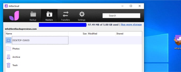
Mengulas Lebih Jauh Tentang Software Disk Yandex – Yandex.Disk adalah layanan cloud yang dibuat oleh Yandex yang memungkinkan pengguna menyimpan